
A Fermi-Hubbard Hamiltonian is not yet a quantum circuit. First, the fermionic modes must be mapped to qubits. Then the circuit must be placed on a real chip. For fermionic simulation, that placement is not a detail. It is part of the algorithm.
The reason is the fermionic sign. When two occupied fermionic modes are exchanged, a minus sign appears. An ordinary qubit SWAP does not know about that sign. This is why we use a fermionic swap: the fSWAP gate.
From sites to qubits
Each Hubbard site has two spin modes: spin-up and spin-down. A chain with 60 sites therefore has 120 fermionic modes. In a Jordan-Wigner style mapping, we place those modes on a line and then map them to qubits.
A useful ordering keeps the two spin modes of the same site close together
\[\{c_{0,\downarrow},c_{0,\uparrow},c_{1,\uparrow},c_{1,\downarrow},c_{2,\downarrow},c_{2,\uparrow},c_{3,\uparrow},c_{3,\downarrow},\ldots\}\rightarrow q_0,q_1,\ldots,q_{2L-1}\]This matters because the onsite interaction is local. If the spin-up and spin-down modes of the same Hubbard site are far apart in the qubit line, we pay for it with extra routing and longer strings.
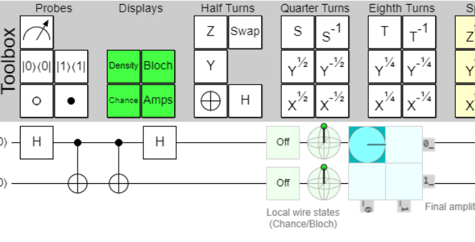
The fSWAP gate
The fSWAP exchanges two fermionic modes and adds the correct sign
\[\mathrm{fSWAP}=\mathrm{SWAP}\cdot\mathrm{CZ}\]As a matrix
\[\mathrm{fSWAP}=\left(\begin{array}{rrrr}1&0&0&0\\0&0&1&0\\0&1&0&0\\0&0&0&-1\end{array}\right)\]The state |01> becomes |10>, and |10> becomes |01>, just as in an ordinary SWAP. The difference is |11>. When both modes are occupied, a minus sign appears. That minus sign is the fermionic anticommutation relation.
Routing becomes physics
In many quantum algorithms, routing feels like a compiler step after the algorithm has already been chosen. For fermionic simulation that view is too simple. An fSWAP layer does two things at once:
- it moves modes so that the next interaction becomes local;
- it preserves the fermionic sign structure.
That is why we cannot simply say: let the compiler add swaps. Here the swaps are not just transport. They are part of the simulated fermionic algebra.
The snake through the chip
IBM processors do not provide a perfect straight line of 120 qubits. The connectivity is limited. The trick is to embed the effective fermion line as a snake through the hardware graph.
A good snake layout tries to do three things at the same time
- keep frequently interacting modes physically close;
- avoid long routing paths;
- avoid bad qubits or bad couplers when calibration data says they are risky.
This is why the Q-CTRL approach does not feel like a generic "press compile" workflow. The physics, mapping, fSWAP layers, hardware connectivity, and error suppression are co-designed.
Why the depth stays low
The resource scaling in the paper explains why this construction is attractive
\[D_{2Q}=5\,n_{\mathrm{step}}+2\qquad N_{2Q}=(5L-2)n_{\mathrm{step}}+2(L-1)-1\]For the smaller 60-qubit / 30-site / 8-step version, this gives
\[D_{2Q}=5\cdot 8+2=42\qquad N_{2Q}=(5\cdot 30-2)\cdot 8+2(30-1)-1=1241\]The two-qubit depth grows with the number of Trotter steps, but not directly with the number of sites. The number of two-qubit gates does grow with the chain length, but only linearly. That is exactly what we want for a large 1D simulation.
The key lesson
The quantum computer does not win here by running an arbitrary circuit faster. The gain comes from translating the Fermi-Hubbard structure so that the hardware almost follows the natural geometry of the problem.
That makes the benchmark more subtle, but also more interesting. The advantage lives in the combination of physics, mapping, layout, and hardware execution.
Sources and project links
- Q-CTRL Fermi-Hubbard paper: https://arxiv.org/abs/2605.04025
- Project repository: https://github.com/BramDo/fermi-hubbard-60q-tdvp