


The 80-qubit experiment is the main result of this series, but it is not the easiest place to learn what an echo or a scrambling front means. This local toy model reduces the same information-flow ideas to two through eight qubits. It runs exactly on a laptop, uses no cloud account, and submits no IBM Quantum or Fire Opal job.
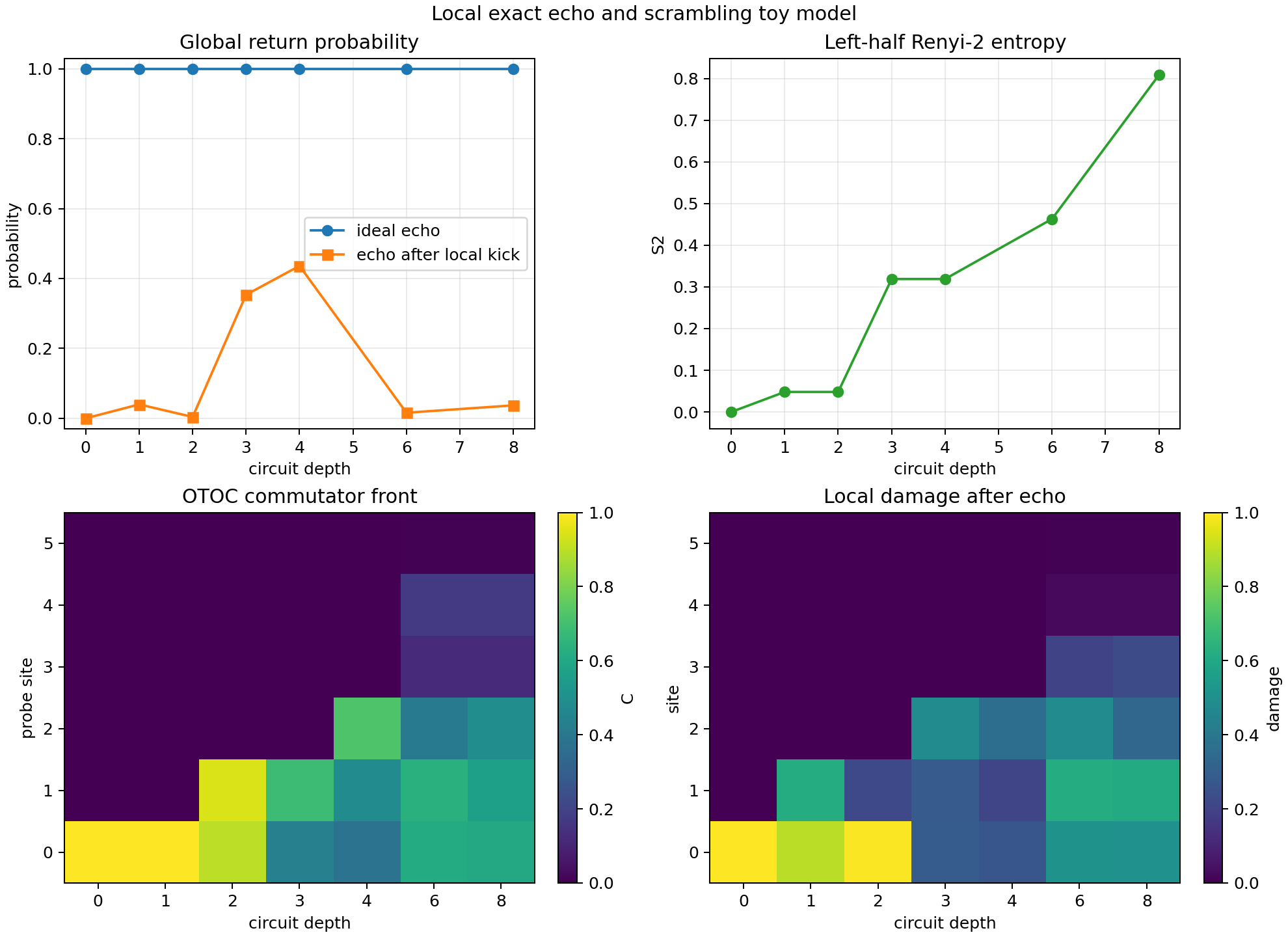
What the model does
- Prepare an
n-qubit product state. - Apply reproducible random single-qubit rotations and alternating nearest-neighbour
CZlayers. - Insert a local Pauli-X kick on a selected site.
- Apply the exact inverse circuit.
- Measure global return, local echo damage, bipartite Renyi-2 entropy, and an OTOC commutator profile.
The implementation deliberately uses dense NumPy matrices. That makes every step inspectable, but it also limits the model to eight qubits. It is an educational exact simulator, not a replacement for the Q80 hardware workflow.
1. Register and scrambling circuit
The initial state is the computational product state
\[|\psi_0\rangle=|0\rangle^{\otimes n}.
\]
At circuit depth d, the forward unitary is
\[U_d=L_{d-1}L_{d-2}\cdots L_0.
\]
Each layer applies independent Rx and Rz rotations followed by CZ gates on alternating even and odd nearest-neighbour bonds. The angles are pseudo-random, while the seed fixes the complete circuit family. Random local circuits are useful minimal models for unitary mixing and operator growth. A shallow run is not claimed to be a proven unitary design.
2. Ideal and perturbed echo
With no kick, forward and inverse evolution cancel exactly:
\[L_0(d)=\left|\langle\psi_0|U_d^\dagger U_d|\psi_0\rangle\right|^2=1.
\]
The perturbed return inserts a local Pauli-X operator on site k:
\[L_X(d)=\left|\langle\psi_0|U_d^\dagger X_k U_d|\psi_0\rangle\right|^2.
\]
This asks whether the original state is globally recovered after scrambling, a local kick, and exact reversal. It is an echo-style operator-insertion return. It is closely related to Loschmidt-echo and fidelity-decay diagnostics, but it is not identical to the common definition based on evolution under two slightly different Hamiltonians.
Yan, Cincio, and Zurek established a direct bridge between the two diagnostic families by showing that an OTOC can be written as a thermal average of Loschmidt-echo signals. That result motivates studying echo and OTOC together here, but it does not make this particular LX(d) estimator identical to the separately calculated Fj(d).
3. Local damage after reversal
The final echo state is
\[|\psi_{\mathrm{echo}}\rangle=U_d^\dagger X_k U_d|\psi_0\rangle.
\]
The model evaluates every local Z observable and reports
\[D_j(d)=\frac{1-\langle\psi_{\mathrm{echo}}|Z_j|\psi_{\mathrm{echo}}\rangle}{2}.
\]
A value of zero means no local deviation from the all-zero reference; one means a complete local inversion. These values are local diagnostics, not a probability distribution, so they do not need to sum to one.
4. Renyi-2 entanglement entropy
After forward evolution, the state is split into a left subsystem A and right subsystem B. Tracing out B gives
\[\rho_A=\operatorname{Tr}_B\left(|\psi_d\rangle\langle\psi_d|\right),
\qquad |\psi_d\rangle=U_d|\psi_0\rangle.
\]
The reported entropy is
\[S_2(A)=-\ln\operatorname{Tr}(\rho_A^2).
\]
A pure product state has S2 = 0. When the two halves become entangled, the reduced-state purity falls and S2 rises. With natural logarithms, the maximum for the smaller half is |A| ln 2. Entanglement growth is evidence of information spreading, but it is not by itself proof of thermalisation, quantum chaos, or quantum advantage.
Nahum, Ruhman, Vijay, and Haah developed the connection between random circuits, operator dynamics, and growing entanglement entropy. Their result supports using S2 as a complementary diagnostic next to the echo and operator front; one small finite circuit realization need not follow a smooth universal growth curve.
5. OTOC operator front
The OTOC diagnostic is separate from the echo kick. It uses a source W = Z_k, local probes V_j = X_j, and the Heisenberg-evolved source
W(d)=U_d^\dagger W U_d.
\]
For every site, the code calculates the infinite-temperature correlator and a normalized commutator proxy:
\[F_j(d)=2^{-n}\operatorname{Tr}\left[W(d)V_jW(d)V_j\right],
\qquad
C_j(d)=\frac{1-\operatorname{Re}F_j(d)}{2}.
\]
At depth zero, the source and probe anticommute on the source site, while probes elsewhere commute. As the Heisenberg operator grows, more distant sites acquire a non-zero value. This produces the operator-front heatmap.
Joshi and colleagues combined almost the same diagnostic family in a ten-qubit trapped-ion experiment: OTOCs from randomized measurements, Rényi entropies, and an explicit analysis of decoherence. Their experiment illustrates why a falling correlator should not be interpreted independently of entanglement and noise.
6. Why the front remains local
Every entangling gate connects neighbouring qubits only. In one brickwork layer, operator support can therefore cross at most one adjacent bond. The model has a strict circuit light cone. This is the discrete-circuit counterpart of the Lieb-Robinson idea that local quantum lattice systems possess an effective maximum speed for information propagation.
Lieb and Robinson formulated the original finite-velocity bound for local quantum spin systems. Roberts and Swingle later connected this locality structure to the butterfly effect: the butterfly velocity describes ballistic operator growth as a state-dependent effective velocity, while the Lieb-Robinson velocity supplies a more general upper bound.
Interference controls the values inside that allowed region. A small value inside the cone does not mean that a site is unreachable; a strict zero outside the cone follows from circuit locality.
7. The black-hole connection
Hawking’s calculation of thermal black-hole emission sharpened the conflict between complete evaporation and unitary quantum evolution. Quantum-information approaches later reframed part of the problem through scrambling: information can remain present in the global quantum state while becoming distributed over many degrees of freedom and locally difficult to recover.
Hayden and Preskill studied information recovery from a rapidly mixing unitary black-hole model. Sekino and Susskind conjectured that black holes are exceptionally fast scramblers. Shenker and Stanford related sensitivity to a small early perturbation to the butterfly effect in holographic black-hole systems. OTOCs then became a standard language for operator growth and this sensitivity.
This toy model borrows only that information structure: a local perturbation, unitary operator spreading, entanglement growth, and an echo that tests recoverability. It contains no spacetime, horizon, gravity, Hawking radiation, black-hole temperature, or evaporation. Its nearest-neighbour chain is also not a black-hole fast-scrambler architecture.
User guide
Requirements
- Python 3.9 or newer
- NumPy
- Matplotlib for the figure
Install on PowerShell
py -m venv .venv-toy
.\.venv-toy\Scripts\Activate.ps1
python -m pip install -r toy_model\requirements.txt
Run the default model
python -m toy_model.black_hole_echoThe default uses six qubits, kick site zero, seed 424242, and depths 0,1,2,3,4,6,8. It writes:
toy_model/output/results.jsonwith all observables, parameters, and theory references;toy_model/output/toy_model.pngwith the four diagnostic panels.
Change the experiment
python -m toy_model.black_hole_echo --qubits 7 --depths 0,1,2,4,6 --kick-site 2 --seed 17Use --output-dir PATH for another output location and --no-plot to produce JSON without Matplotlib.
Run the tests
python -m unittest tests.test_toy_model -vThe tests check the exact depth-zero reference, physical numerical bounds, deterministic reproduction, argument validation, and the exported scientific references.
Default numerical result
| Depth | Ideal echo | Kicked echo | Renyi-2 | Maximum OTOC C | Maximum local damage |
|---|---|---|---|---|---|
| 0 | 1.000000 | 0.000000 | 0.0000 | 1.000000 | 1.000000 |
| 1 | 1.000000 | 0.039796 | 0.0480 | 1.000000 | 0.895577 |
| 2 | 1.000000 | 0.003908 | 0.0480 | 0.943543 | 0.996089 |
| 3 | 1.000000 | 0.353363 | 0.3190 | 0.684813 | 0.483125 |
| 4 | 1.000000 | 0.436055 | 0.3190 | 0.725132 | 0.361385 |
| 6 | 1.000000 | 0.015995 | 0.4630 | 0.635537 | 0.618656 |
| 8 | 1.000000 | 0.037037 | 0.8082 | 0.604576 | 0.612326 |
The important sanity check is exact inversion: the ideal echo remains one at every depth. The entropy rises overall and the heatmaps reveal spatial structure. The non-monotonic kicked return is expected for one finite random circuit realization and should not be read as a smooth thermodynamic decay law.
Limits
- Dense matrices scale as
2^n x 2^n, so the CLI is intentionally capped at eight qubits. - The model has no shots, hardware noise, readout mitigation, or zero-noise extrapolation.
- The observables are educational diagnostics and are not numerically identical to every q14-q80 hardware observable in the project.
- The result is not evidence for quantum advantage because the entire toy model is classically simulated.
- The result is not an astrophysical black-hole simulation.
Scientific sources
- S. W. Hawking, Particle creation by black holes, Communications in Mathematical Physics 43, 199-220 (1975).
- T. Gorin, T. Prosen, T. H. Seligman and M. Znidaric, Dynamics of Loschmidt echoes and fidelity decay, Physics Reports 435, 33-156 (2006).
- B. Yan, L. Cincio and W. H. Zurek, Information Scrambling and Loschmidt Echo, Physical Review Letters 124, 160603 (2020).
- P. Hayden and J. Preskill, Black holes as mirrors: quantum information in random subsystems, JHEP 2007(09), 120.
- Y. Sekino and L. Susskind, Fast Scramblers, JHEP 2008(10), 065.
- S. H. Shenker and D. Stanford, Black holes and the butterfly effect, JHEP 2014(03), 067.
- E. H. Lieb and D. W. Robinson, The Finite Group Velocity of Quantum Spin Systems, Communications in Mathematical Physics 28, 251-257 (1972).
- D. A. Roberts and B. Swingle, Lieb-Robinson Bound and the Butterfly Effect in Quantum Field Theories, Physical Review Letters 117, 091602 (2016).
- A. Nahum, J. Ruhman, S. Vijay and J. Haah, Quantum Entanglement Growth under Random Unitary Dynamics, Physical Review X 7, 031016 (2017).
- A. Nahum, S. Vijay and J. Haah, Operator Spreading in Random Unitary Circuits, Physical Review X 8, 021014 (2018).
- B. Nachtergaele, R. Sims and A. Young, Quasi-Locality Bounds for Quantum Lattice Systems. Part I (2018).
- M. K. Joshi et al., Quantum Information Scrambling in a Trapped-Ion Quantum Simulator with Tunable Range Interactions, Physical Review Letters 124, 240505 (2020).
- A. W. Harrow and R. A. Low, Random Quantum Circuits are Approximate 2-designs, Communications in Mathematical Physics 291, 257-302 (2009).
- I. Garcia-Mata, R. A. Jalabert and D. A. Wisniacki, Out-of-time-order correlations and quantum chaos, Scholarpedia 18(4), 55237 (2023).