


Scope of this part: this part explains how to read the charge and spin heatmaps. Part 9 uses those observables for a different question: when do a digital processor and a cold-atom setup count as implementations of the same Hubbard experiment?
A table of RMSE values is useful, but it is not a physical picture. For a material-like story, we want to see where something happens in the chain and how it changes in time. That is why heatmaps are important.
In this project series, the heatmaps use
- x-axis: site position in the 1D chain;
- y-axis: Trotter step or model time;
- color: charge or spin.
The time relation is
\[t=n_{\mathrm{step}}\Delta t\qquad \Delta t=0.2,\quad n_{\mathrm{step}}=30,\quad t=6\]The observables are
\[n_\uparrow(i)=\langle n_{i,\uparrow}\rangle,\quad n_\downarrow(i)=\langle n_{i,\downarrow}\rangle\\ \mathrm{charge}(i)=n_\uparrow(i)+n_\downarrow(i)\\ \mathrm{spin}(i)=n_\uparrow(i)-n_\downarrow(i)\\ D(i)=\langle n_{i,\uparrow}n_{i,\downarrow}\rangle\]Charge heatmap
The charge heatmap shows n_up + n_down for each site. At half filling, many sites should remain around charge 1. Deviations show local redistribution of particles.
In the local 120-qubit hardware data, the pattern is not perfectly smooth. That is expected. The data contains real hardware noise, readout errors, finite shots, and layout asymmetry. Even so, the picture is useful: it shows whether the chain roughly preserves its filling and where the largest local deviations appear.
Spin heatmap
The spin heatmap shows n_up - n_down. This observable is more sensitive to state preparation and noise. In our data, the spin structure decays more quickly toward smaller values. That is consistent with dephasing and relaxation in a noisy digital simulation.
This does not mean that the hardware perfectly reproduces closed-system Hubbard dynamics. It means that the observables contain enough structure to build a material-like view.
Comparison with real experiments
There are real 1D Fermi-Hubbard experiments with ultracold atoms in optical lattices. With a quantum gas microscope, groups can perform site-resolved measurements as a function of evolution time.
A well-known experimental figure shows a local quench in the center of the chain. That plot is nearly symmetric: an excitation starts around i = 0 and moves left and right.
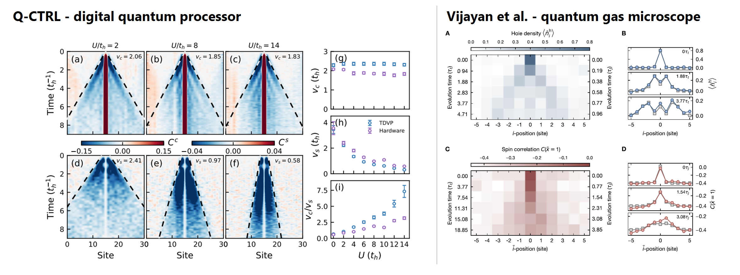
Our plot is different. We show a 60-site digital evolution, not a local center-quench. Site 46 is interesting because the Q-CTRL paper discusses that site, but it is not a symmetry center. The IBM hardware layout itself is also not left-right symmetric.
Therefore the right formulation is
Our heatmap is comparable as a measurement type and model language, but not as an identical experimental configuration.
What does the heatmap teach?
The heatmap shows three things at once
- the physical quantities: charge and spin along a 1D chain;
- the digital evolution: different Trotter steps as time points;
- the hardware reality: noise, readout, and layout asymmetry.
That is why the plot is useful. It is not only a nice figure. It shows where the quantum run is physically interpretable and where caution is still needed.
Why asymmetry is not fatal
A symmetric cold-atom local-quench plot and our asymmetric 60-site hardware plot answer different questions. The cold-atom plot asks: how does a local excitation move through a chain? Our plot asks: what site-resolved observables do we obtain from a large digital Hubbard run?
Those are related questions, but not the same one.
The asymmetry therefore does not make the data useless. It only means that we should not sell it as a symmetric quench experiment.
The best role of the heatmap
The heatmap is a bridge figure. It makes the quantum run understandable for readers who do not want to look only at circuits or RMSE tables. It shows that the output of a quantum processor can be read as a 1D material-like image.
That is a strong communication step, as long as the claim boundaries remain clear.
Sources and project links
- Project repository: https://github.com/BramDo/fermi-hubbard-60q-tdvp
- Time-resolved 1D Hubbard cold-atom experiment: https://arxiv.org/abs/1905.13638
- Q-CTRL Fermi-Hubbard paper: https://arxiv.org/abs/2605.04025