From toy model to 51 qubits: where does quantum advantage begin?

Nederlands

Part 6 of the Floquet-Ising series: from two qubits to prethermal oscillations

The two-qubit model is exact, fast, and fully controllable. That is scientifically useful, but computationally unimpressive. Quantum advantage becomes a meaningful question only when a quantum processor performs a precisely defined task for which the best credible classical route is insufficient at the same accuracy.

The validation ladder

The repository does not jump directly from two to 51 qubits. Each step adds part of the real structure:

Step	What is added?	What remains controllable?
2 qubits	one ZZ bond, three Floquet layers	all amplitudes and matrices
4 qubits	all three edge colours, one genuine distance-three pair	exact statevector
7 qubits	four official ZZd3 pairs	exact statevector
12 qubits	closed tracker loop, twelve pairs	exact trajectory
21 qubits	induced heavy-hex patch, 26 pairs	exact reference plus MPS sweep
51 qubits	full public tracker, 86 pairs	hardware, mitigation, and classical approximations

This ladder tests more than performance. It also reveals semantic errors: incorrect qubit order, a swapped bond-colour pattern, or averaging over the wrong correlation pairs.

Why a statevector explodes

A dense N-qubit state contains 2 to the power N complex amplitudes. At 21 qubits, that is more than two million amplitudes, and a carefully designed exact calculation is still feasible. At 51 qubits, there are approximately 2.25 times 10 to the power 15 amplitudes. Even at sixteen bytes per amplitude, this requires tens of petabytes, before intermediate results.

MPS: compression based on entanglement

A matrix product state replaces the amplitude tensor with a chain of smaller tensors. The internal bond dimension chi limits how many Schmidt coefficients are retained across each cut. Roughly, the entanglement entropy cannot exceed log2 chi without truncation.

\[
S_{\mathrm{cut}}\leq \log_2\chi.
\]

On our 21-qubit patch, we ran a sweep with chi = 32, 64, 128, and 256. The errors relative to the exact trajectory decrease systematically. At chi = 256, however, the maximum errors remain approximately 0.0236 for magnetization and 0.0152 for the average ZZd3. Every run reaches its bond-dimension cap. The correct conclusion is therefore: improving, but not yet converged.

A fast runtime does not make an unconverged result exact. Conversely, classical nonconvergence does not automatically mean that the quantum result is correct.

The 51-qubit task

The public tracker contains 16 Floquet cycles, 56 RZZ bonds per cycle, and 86 distance-three ZZ pairs. The measured task is not to reconstruct the full state, but to estimate a specific average:

\[
\overline{ZZ}_{d=3}=
\frac{1}{86}\sum_{(i,j)\in\mathcal{P}_{d=3}}
\langle Z_iZ_j\rangle.
\]

This distinction matters. A classical method may compute the observable directly and need not store every amplitude. Fair advantage comparisons should therefore use the best observable-specific algorithms, such as tensor networks or sparse Pauli paths, rather than only a naive statevector.

What makes the paper stronger than a single hardware curve

The paper compares QESEM results with PEPS-BP, sparse Pauli paths, and statevector projections. Early cycles are used to test overlap and convergence. At greater depth, the classical approximations diverge or reach resource limits. At the same time, the quantum results are checked using multiple mitigation routes and hardware platforms.

The paper’s conclusion is specific: for the studied prethermal dynamics and precision, the error-mitigated quantum route reaches a regime beyond the controlled classical methods the authors executed. That is stronger than saying that 51 qubits are generally impossible to simulate classically.

What the full IBM Fez replication now shows

We have now run the public 51-qubit circuit twice in full, from cycle 1 through 16, on ibm_fez, using the same physical layout and 512 shots per cycle per arm. The figure shows the preregistered primary route: the raw measurement after local M3 readout mitigation. We therefore compare two independent hardware measurements of exactly the same observable without changing processor or qubit mapping.

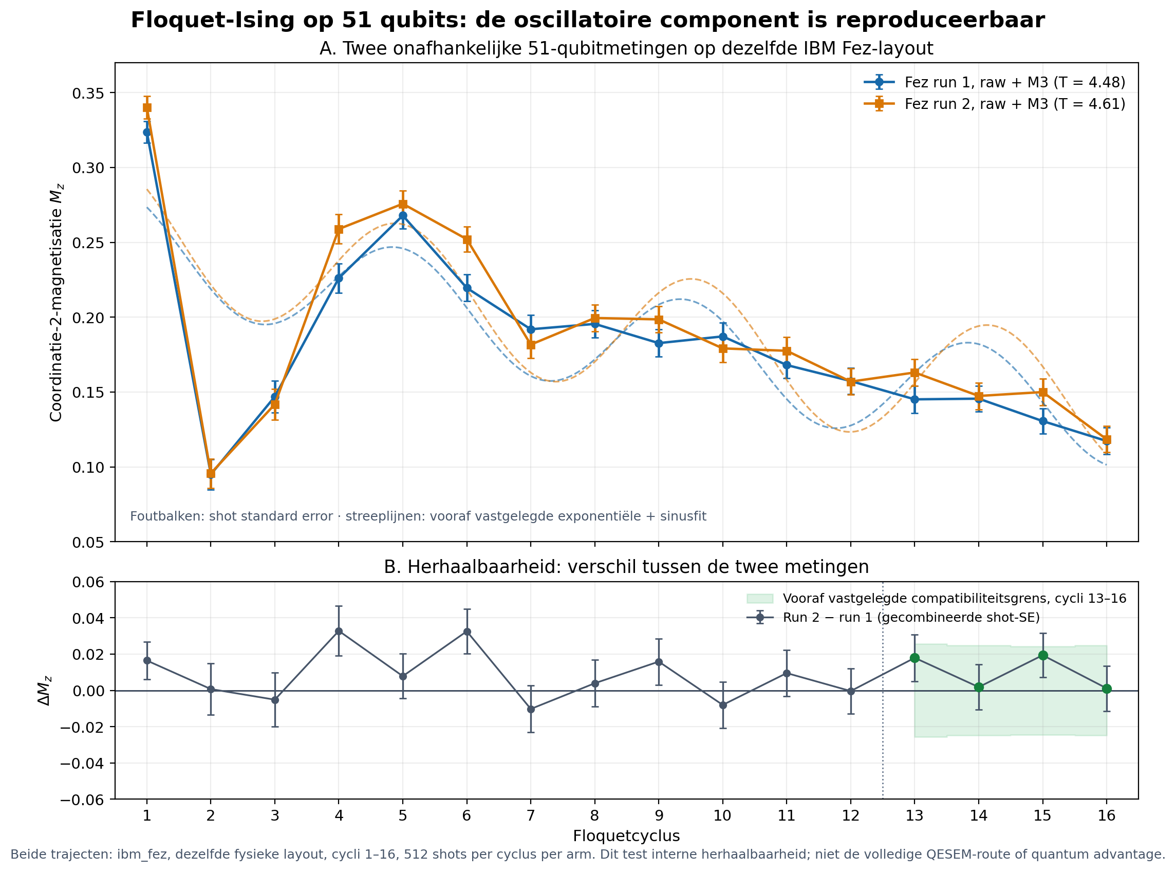
The two curves follow the same troughs and peaks. The fitted period shifts only from 4.48 to 4.61 cycles: a difference of 0.13 cycle, well within the preregistered repeatability threshold of 0.5 cycle. All four late points, cycles 13–16, are also compatible under the preregistered pointwise test. For raw+M3, the second run additionally shows a strong preference for the oscillatory model over a purely monotonic decay curve (Delta AICc approximately 168.6; amplitude divided by fit error approximately 13.4).

This sharpens the conclusion: an approximately period-four magnetic oscillatory component is internally reproducible for this 51-qubit task. The stricter rule requiring at least three of the four raw/XY4/M3 views to pass simultaneously remains negative; repeatability is strongest for the preregistered raw+M3 route and is not uniform across every mitigation view. This is therefore not yet evidence of advantage: it does not establish exact accuracy at cycle 16, fully reproduce QESEM, or independently demonstrate quantum advantage.

A checklist for quantum advantage

1. Same task: identical circuit, parameters, cycles, and observable.
2. Same accuracy: explicit statistical and systematic uncertainties.
3. Quantum validation: independent mitigation views, repetitions, and calibration audit.
4. Classical convergence: systematic scaling of bond dimension, truncation, or term cutoff.
5. Resources: clearly defined QPU sampling, calibration, preprocessing, and classical computation time.
6. Claim boundary: advantage for this estimator, not for all quantum dynamics.

The final lesson

The toy model and the 51-qubit experiment are not rivals. The toy model provides understanding and an exact software oracle. The larger patches test geometry and classical approximations. The hardware reaches the scale at which the physical question becomes interesting. Only the full chain supports a reliable scientific conclusion.

The most valuable result of the series is therefore not a single speed figure. It is a method: begin with a fully understandable model, add complexity in controlled steps, and require every larger claim to rest on a comparison that answers the same question.

Sources and reproduction

1. FLOQUET-QEM repository.
2. 21-qubit MPS convergence report.
3. E. Leviatan et al., paper and classical resource comparison.