


Edukaizen

Menu
  • News
  • Hubbard
    • Hubbard 1D
      • Part 1: 1D Hubbard model
      • Part 2: Snake layout and fSWAP
      • Part 3: Qiskit and Fire Opal
      • Part 4: 120-qubit run
      • Part 5: Time-to-answer
      • Part 6: Tensor networks
      • Part 7: Majorana propagation
      • Part 8: Reading heatmaps
      • Part 9: Digital vs cold-atom labs
      • Part 10: Official Monoprop benchmark
    • Hubbard 2D
      • Part 1: 1D to 2D
      • Part 2: Cuprates
      • Part 3: 3×3
      • Part 4: Time
      • Part 5: 4×4
      • Part 6: 6×6 Fez
    • 2D Local Quantum Advantage
      • Deel 1: Doel en budget
      • Deel 2: Fermionmodel
      • Deel 3: Mapping en diepte
      • Deel 4: Pilots en shots
      • Deel 5: Foutmitigatie
      • Deel 6: 6×6-resultaten
      • Deel 7: Circa 20x
      • Deel 8: Google en Bonsai
      • Deel 9: Volgende stap
  • Hadron
    • Part 1: Hadron on a quantum processor
    • Part 2: Quarks and confinement
    • Part 3: SU(2) and LSH
    • Part 4: Hamiltonian and circuit
    • Part 5: Fire Opal
    • Part 6: Classical simulations
    • Part 7: Quantum advantage
  • Black Hole OLE
    • Part 1: What we ran
    • Part 2: How OLE works
    • Part 3: Fire Opal and Kingston
    • Part 4: The tensor-network challenge
    • Part 5: Hawking and scrambling
    • Part 6: What the result proves
    • Part 7: Local toy model
    • Part 8: QGSS26 compatibility
  • Random Graph
    • Start here
    • Part 1: Theory
    • Part 2: Circuit
    • Part 3: Qiskit
    • Part 4: Complexity
    • Part 5: Verification
    • Part 6: Workflow
    • Part 7: Conclusion
  • Floquet-Ising
    • Part 1: Floquet physics
    • Part 2: Ising cycle
    • Part 3: Two-qubit toy model
    • Part 4: Oscillation and entanglement
    • Part 5: Noise and error mitigation
    • Part 6: Toward 51 qubits
  • XXZham
    • Part 1: The XXZ model and imbalance
    • Part 2: From dynamics to a quantum circuit
    • Part 3: The classical simulation methods
    • Part 4: Error mitigation on real hardware
    • Part 5: Results and the classical comparison
    • Part 6: Original study and next steps
  • Work
    • QOS QML
      • Tutorial: UMI counts to a four-qubit circuit
      • Part 1: The QML task
      • Part 2: QOS theory
      • Part 3: Gene expression to 40 qubits
      • Part 4: JAX to hardware
      • Part 5: Readout and classifier
      • Part 6: 40-qubit result
      • Part 7: Route to quantum advantage
      • Part 8: 60-qubit result
    • Quantum Gold
      • Part 1: Why gold is a relativistic quantum problem
      • Part 2: Why the 2025 gold VQE study stalled
      • Part 3: From QE and spin–orbit coupling to Qiskit
      • Part 4: Twelve gold spinor modes on four qubits
      • Part 5: The 24-qubit route: an active window for transport
      • Part 6: 24 qubits on IBM and with Fire Opal
      • Part 7: The road to quantum advantage for gold
      • Part 8: 24 gold spinor modes on IBM with ZNE-PEA
      • Part 9: Forced gold colour on 56 qubits
    • HaPPY Gravity
      • Part 1: Gravity as a phase gate
      • Part 2: Bosons and convergence
      • Part 3: The dynamic HaPPY benchmark
      • Part 4: The N=145 classical audit
      • Part 5: MPS and Majorana baselines
      • Part 6: PEA/ZNE and the decisive test
    • Fibonacci Anyons
      • Part 1: Fusion and braiding
      • Part 2: The 3/5/9-qubit ladder
      • Part 3: Why nine qubits were too deep
      • Part 4: Structure-aware simplification
      • Part 5: IBM hardware diagnostic
      • Part 6: Results and open questions
  • Advantage List
  • Contact
Menu

Part 5: Results and the classical comparison

NederlandsEnglish

XXZham / Part 5 / 6

Our own measurement alongside classical calculations

The hardware measurement ran on IBM Kingston, Heron R2, using the Open plan. It included 31 N80 points and three N12 controls. For the errors below, we consistently use the same reference: the arithmetic mean of the original TEBD and TDVP curves. That mean is not an exact solution.
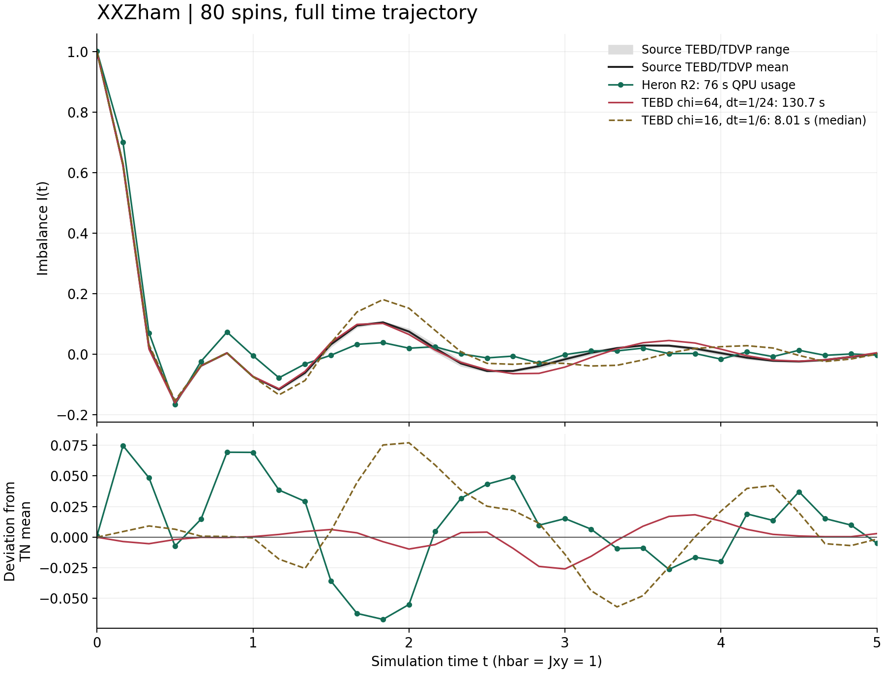
Full imbalance trajectory for 80 spins: Heron R2, two local TEBD settings, and the original TEBD and TDVP references.
Top: all 31 time points. Bottom: deviations from the TN mean. The grey band shows the difference between the two source methods, not a statistical confidence interval. The timings measure different resources, not total turnaround time.
Calculation Time RMSE Maximum deviation
Heron R2, with mitigation 76 s QPU usage 0.03694 0.07476
Local TEBD, chi=64, dt=1/24 130.7 s execution 0.00951 0.02589

The ratio 130.7/76 is approximately 1.72. Our quantum run used fewer QPU seconds than this refined classical run required in CPU execution seconds, but with a larger deviation. This is a concrete comparison of two measured settings, not a demonstrated speedup at matched quality. QPU usage here also includes the small control circuits; it is not the same metric as CPU execution time or total turnaround time.

IBM separately recorded 66.93 seconds of circuit execution. Approximately 46 minutes elapsed between submission and completion; local preparation took 56.17 seconds. Including process startup and preparation, the classical run took 133.95 seconds. The classical computer was an AMD Ryzen 5 3500U, using one CPU thread in our established Qiskit/Quimb environment. This is not a comparison with the fastest available classical hardware.

There is also a much cheaper classical approximation: chi=16 and dt=1/6 computed the same 31 time points in a median of 8.01 seconds across five runs. It satisfied our original, relatively loose error criteria against both source curves, but failed a separate convergence test. The refined chi=64 run has not been shown to be converged either. All nine convergence runs together took 446.2 seconds. That total validation time is not the time needed for a single classical simulation.

A later quantum attempt with a 40-second limit was terminated without producing a complete curve. The successful demonstration in this article is the 76-second run, not that interrupted attempt.

Previous: part 4OverviewNext: part 6

Recent Posts

  • Quantum computing-nieuws — 18 september 2026
  • A Call to Qiskit Advocates: Help Test Quantum Advantage
  • Quantum computing-nieuws — 11 september 2026
  • Quantum computing-nieuws — 4 september 2026
  • Quantum computing-nieuws — 28 augustus 2026

Recent Comments

  1. XXZham: simulating 80 spins with a NISQ quantum computer - Edukaizen on XXZham: quantumsimulatie van 80 spins

Archives

  • September 2026
  • August 2026
  • July 2026
  • May 2026
  • March 2026
  • February 2026
  • September 2024

Categories

  • 10
  • Quantum Computing
  • Uncategorized
©2026 Edukaizen | Theme by SuperbThemes