


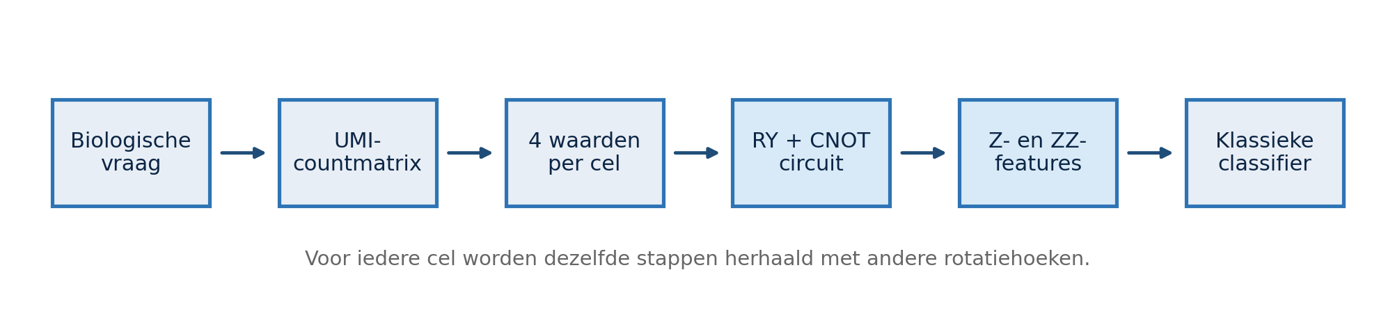
How does a row of gene-expression data become an executable quantum circuit? In this guide, we follow one real PBMC68k cell from raw UMI counts to four rotation angles, a small Qiskit circuit, eight quantum features, and a classical classifier.
This is deliberately a beginner model. It runs on a four-qubit simulator, uses only 16 training and 16 test cells, and makes no quantum-advantage claim. Its purpose is to make the complete translation chain visible and reproducible.
1. The task: distinguish two immune-cell types
In our loader, the PBMC68k dataset contains 68,579 cells and 32,738 genes. A row is one cell, a column is one gene, and every matrix value is a molecule count. We select two cell types:
CD4+/CD25 T Reg;CD4+/CD45RO+ Memory.
The selected binary subset contains 9,248 cells. For the educational experiment, fixed seed 11 selects eight training and eight test cells per class. Training and test sets do not overlap.
The task is therefore not to look up a gene. It is:
gene-expression profile of one cell -> quantum feature map -> predicted cell type2. What is a UMI count?
UMI means Unique Molecular Identifier. Before amplification in the laboratory, every captured RNA molecule receives a short barcode. Reads with the same cell barcode, gene, and UMI are probably copies of the same original molecule, so they count together as one molecule.
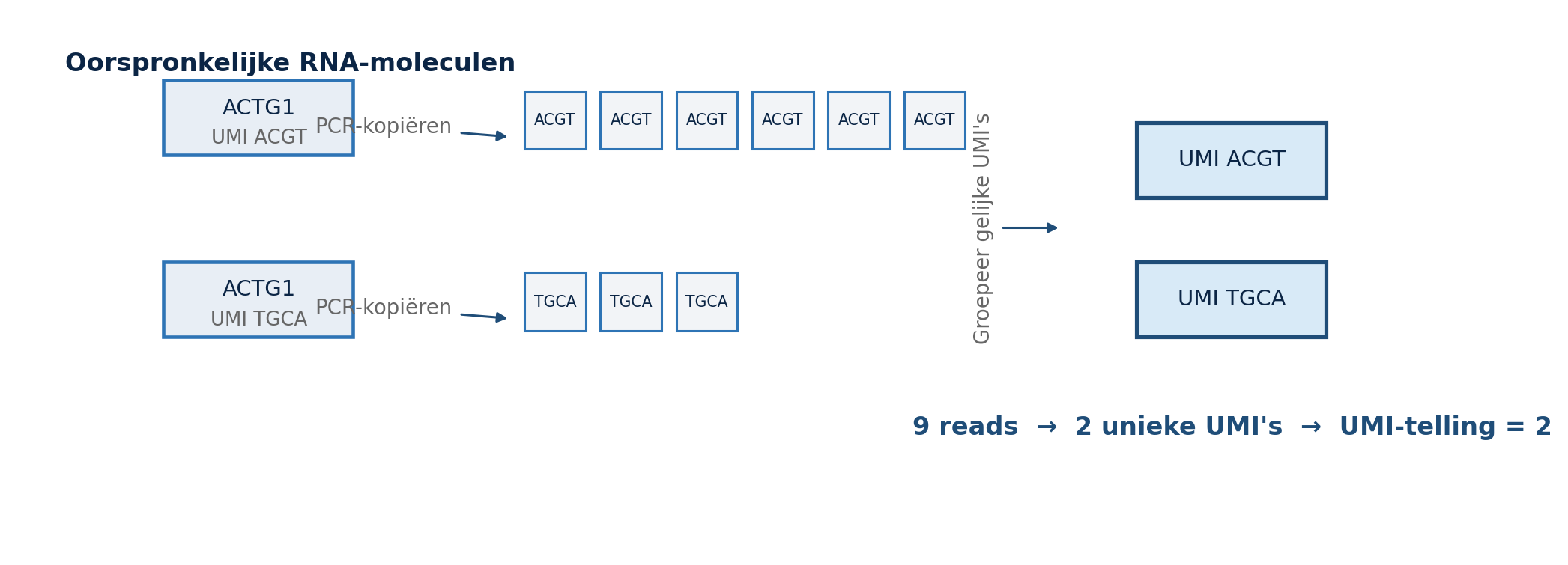
A cell with five reads carrying UMI ACGT and four reads carrying UMI TGCA therefore has nine reads for that gene, but only two distinct UMIs. The resulting count matrix is sparse and contains non-negative integers. A zero means that no molecule was detected; it does not prove that the gene was biologically absent.
3. Split first, then learn every choice
All data-dependent choices are made from the sixteen training cells only:
- select four genes without using labels;
- learn normalization and scaling parameters;
- calculate quantum features for the training set;
- train the classical classifier;
- only then evaluate the sixteen held-out test cells.
Among genes with a useful detection frequency, the script selects the four largest training variances. For seed 11 these are:
| Qubit | Gene | Detection in training | Training mean | Training standard deviation |
|---|---|---|---|---|
| 0 | IER2 | 0.6250 | 1.724827 | 1.482075 |
| 1 | ACTG1 | 0.7500 | 2.261162 | 1.377323 |
| 2 | LIMD2 | 0.5625 | 1.427313 | 1.354013 |
| 3 | GLTSCR2 | 0.7500 | 2.266142 | 1.349629 |
The order matters: selecting genes with knowledge of test labels, or fitting the scale on test values, would introduce data leakage.
4. From a raw UMI count to a rotation angle
Cells do not all contain the same total amount of measured RNA. We therefore divide the count for gene g by all UMIs in cell i, scale to 10,000, and apply log1p:
We then use only the training mean and training standard deviation:
\[z_{ig}=\frac{\ell_{ig}-\mu_g^{\mathrm{train}}}{\sigma_g^{\mathrm{train}}}.\]The z-score is clipped to [-3,3] and converted into an angle:
Every angle therefore lies between -pi and pi.
The first real training cell has label CD4+/CD45RO+ Memory, contains 2,010 UMIs in total, and produces:
| Gene | Raw UMI | log1p |
z-score | Angle in radians |
|---|---|---|---|---|
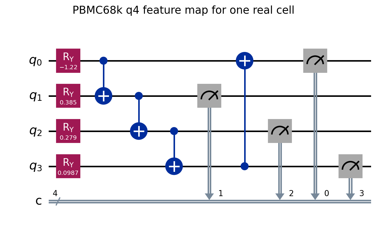
| IER2 | 0 | 0.000000 | -1.163792 | -1.218720 |
| ACTG1 | 3 | 2.767914 | 0.367925 | 0.385290 |
| LIMD2 | 1 | 1.787605 | 0.266092 | 0.278651 |
| GLTSCR2 | 2 | 2.393362 | 0.094263 | 0.098712 |
5. The four-qubit circuit
We start in basis state |0000>. Each angle controls one RY gate. Four CNOT gates then connect the qubits in a ring: 0->1, 1->2, 2->3, and 3->0.
The Y rotation has matrix:
\[R_Y(\theta)=\begin{pmatrix}\cos(\theta/2)&-\sin(\theta/2)\\ \sin(\theta/2)&\cos(\theta/2)\end{pmatrix}.\]For four qubits, the rotation layer is the tensor product:
\[R=R_Y(\theta_3)\otimes R_Y(\theta_2)\otimes R_Y(\theta_1)\otimes R_Y(\theta_0).\]The complete cell-dependent operation is:
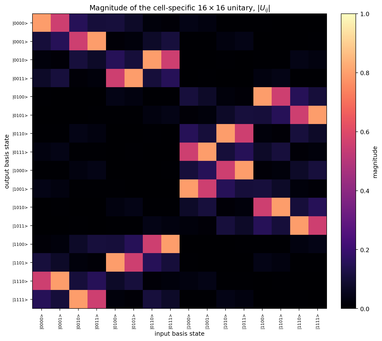
\[U(\theta)=\operatorname{CNOT}_{3\rightarrow0}\operatorname{CNOT}_{2\rightarrow3}\operatorname{CNOT}_{1\rightarrow2}\operatorname{CNOT}_{0\rightarrow1}R.\]Four qubits have 2^4 = 16 basis states, so U is a 16 x 16 matrix. The numerical check gives ||U^dagger U-I||_F = 1.11 x 10^-15: within rounding error, the matrix is unitary.
6. From state to measurement probabilities
The circuit creates the state:
\[|\psi(\theta)\rangle=U(\theta)|0000\rangle=\sum_{b=0}^{15}a_b|b\rangle.\]According to the Born rule, the probability of bit string b is:
For the example cell, the largest ideal probabilities are:
Basis state q3q2q1q0 |
Probability |
|---|---|
0000 |
0.633736 |
1110 |
0.308730 |
1111 |
0.024114 |
1101 |
0.012463 |
Qiskit displays bit strings as q3 q2 q1 q0; qubit 0 is therefore on the right.
7. Eight quantum features from bit strings
For a measured bit b_q, we use the Z eigenvalue (-1)^{b_q}. The single- and two-qubit expectation values are:
\[\langle Z_q\rangle=\sum_b p_b(-1)^{b_q},\]
\[\langle Z_qZ_r\rangle=\sum_b p_b(-1)^{b_q+b_r}.\]
Each cell produces four single-qubit Z features and four neighbouring ZZ features:
\[f(x)=(\langle Z_0\rangle,\langle Z_1\rangle,\langle Z_2\rangle,\langle Z_3\rangle,\langle Z_0Z_1\rangle,\langle Z_1Z_2\rangle,\langle Z_2Z_3\rangle,\langle Z_3Z_0\rangle).\]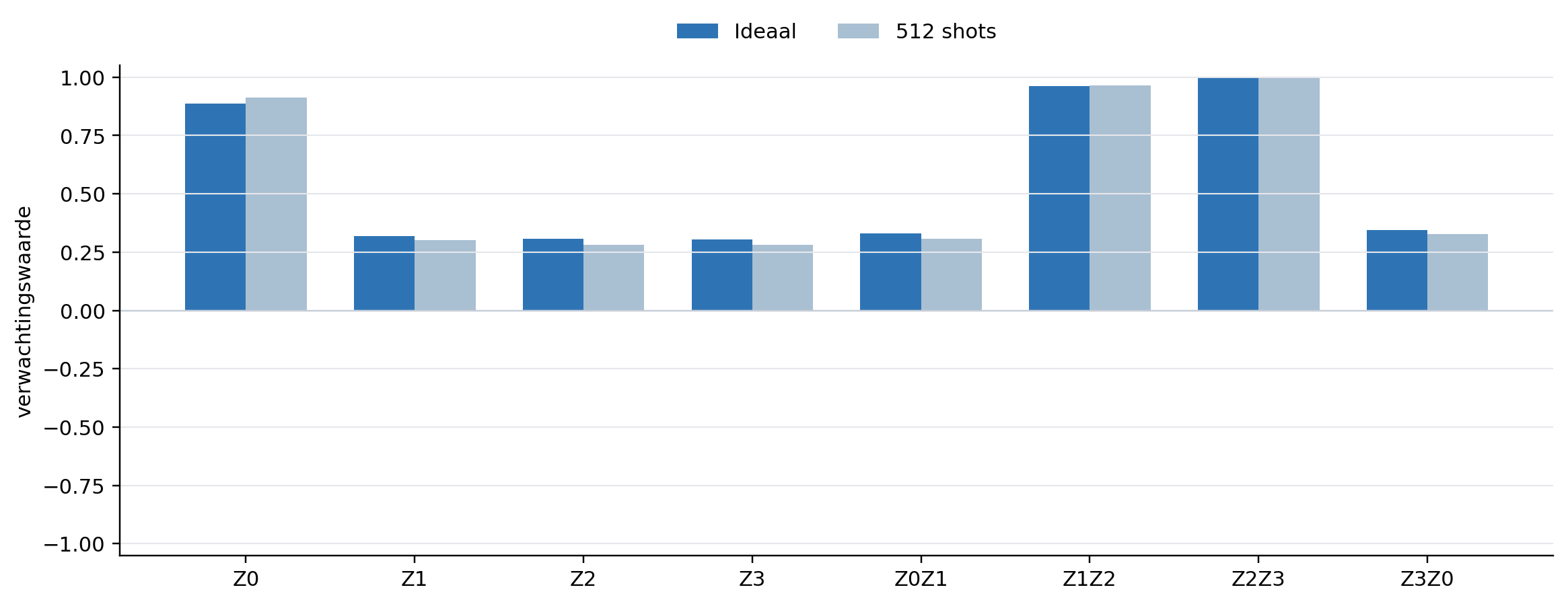
| Feature | Ideal | 512 shots |
|---|---|---|
| Z0 | 0.886607 | 0.914063 |
| Z1 | 0.319566 | 0.300781 |
| Z2 | 0.307240 | 0.281250 |
| Z3 | 0.305744 | 0.281250 |
| Z0Z1 | 0.329931 | 0.308594 |
| Z1Z2 | 0.961427 | 0.964844 |
| Z2Z3 | 0.995132 | 1.000000 |
| Z3Z0 | 0.344847 | 0.328125 |
The difference between ideal values and 512-shot estimates is ordinary sampling noise. More shots reduce the average error, but require more circuit executions.
8. Why a classical classifier is still required
The quantum circuit produces features; it does not choose the final label by itself. Using the sixteen training labels, a classical logistic-regression model learns:
\[P(y=+1\mid f)=\sigma(w^Tf+b), \qquad \sigma(a)=\frac{1}{1+e^{-a}}.\]On the sixteen held-out test cells, the result is:
| Model | Correct | Balanced accuracy |
|---|---|---|
| Four-qubit quantum features | 7/16 | 0.4375 |
| Classical, using the same four genes | 9/16 | 0.5625 |
This is a successful reproducibility and teaching demonstration, but not a performance advantage. A good QML tutorial should report an unfavourable classical comparison honestly.
9. Run it yourself
The simulator route uses no IBM or Fire Opal quantum time:
/home/bram/.venvs/qiskit/bin/python \
  qiskit_qos_pbmc68k_q4_educational.py \
  --shots 512 \
  --json-out output/pbmc68k_q4_educational.json
Regenerate the tables, circuit drawing, and matrices with:
/home/bram/.venvs/qiskit/bin/python \
  qiskit_qos_pbmc68k_q4_explain.py \
  --shots 512 \
  --output-dir docs/beginner/assets
The complete source code and all fixed artifacts are available on GitHub. A downloadable DOCX guide is available there as well.
10. Relationship to Quantum Oracle Sketching
This PBMC68k beginner model is not a literal QOS implementation. It uses four classically prepared rotation angles, a fixed CNOT ring, and Z/ZZ readout. It is a conventional small quantum feature map.
The repository also contains a separate four-qubit hardware pilot that does port the official q_state_sketch_flat sampling kernel to Qiskit. That pilot implements only one QOS building block, not the complete QOS/QSVT classification chain.
| Route | Purpose | Literal QOS kernel? | Claim boundary |
|---|---|---|---|
| Four-qubit PBMC68k beginner model | Learn the translation from UMI data to circuit and classifier | No | No advantage claim |
| Four-qubit flat-QOS hardware pilot | Test the official sampling sketch on hardware | Yes, one primitive | No complete QOS classifier |
| 60-qubit PBMC68k pilot | Test a wide real-data hardware feature map | No, QOS-inspired | Only a bounded local timing claim |
Sources
- Kivioja et al., Counting absolute numbers of molecules using unique molecular identifiers, Nature Methods 9, 72-74 (2012).
- Zheng et al., Massively parallel digital transcriptional profiling of single cells, Nature Communications 8, 14049 (2017).
- IBM Quantum documentation for the RY gate.
- IBM Quantum documentation for bit ordering.
- Havlicek et al., Supervised learning with quantum-enhanced feature spaces, Nature 567, 209-212 (2019).
- Zhao et al., Exponential quantum advantage in processing massive classical data, arXiv preprint (2026).
- 10x Genomics PBMC68k count matrix.